An Introduction to Machine Learning

If you’ve seen any technology news in the past couple of years, it was probably a headline having something to do with computers able to achieve feats previously thought impossible. Driving cars, diagnosing patients, or beating world champions at complex strategy board games, have all be done. All of these tasks are being done with an exploding branch of computer science called artificial intelligence. In this post I’ll look at a subset of AI called machine learning and breakdown one of the simpler algorithms called linear regression.

Machine learning is a category of algorithms that can “learn” from data. In other words, if they’re given a particular task, \(T\), machine learning algorithms can improve at that task (to some limit) given experiences, \(E\).

Linear Regression

The algorithm that we’ll look at is called linear regression. At its heart, linear regression is a “line-fitting” algorithm: given some data that seems to form some kind of line on a graph, we want to derive an equation that describes that line. With such an equation, we can make predictions about new values that are outside out initial dataset.

To put it in more concrete terms, let’s say we wanted to build a model that could predict house prices in a certain area. If we plotted the size of the the house (in square feet) compared to the price that the house sold for, we would likely see some kind of linear distribution of the data points. Using linear regression, we could find the equation of that line, and then predict how much money we think a new house will sell for given its square footage.

In reality, most problems like this are much more complex than this simple example. For instance, houses can have dozens of factors (or “features”) that contribute to their selling price, like the number of bedrooms, school district, and so on. Despite this complexity in the real world, we can look past the specific and learn the principles that form the foundation of these complicated models.

Case Study

For our example, let’s say we have the following data:

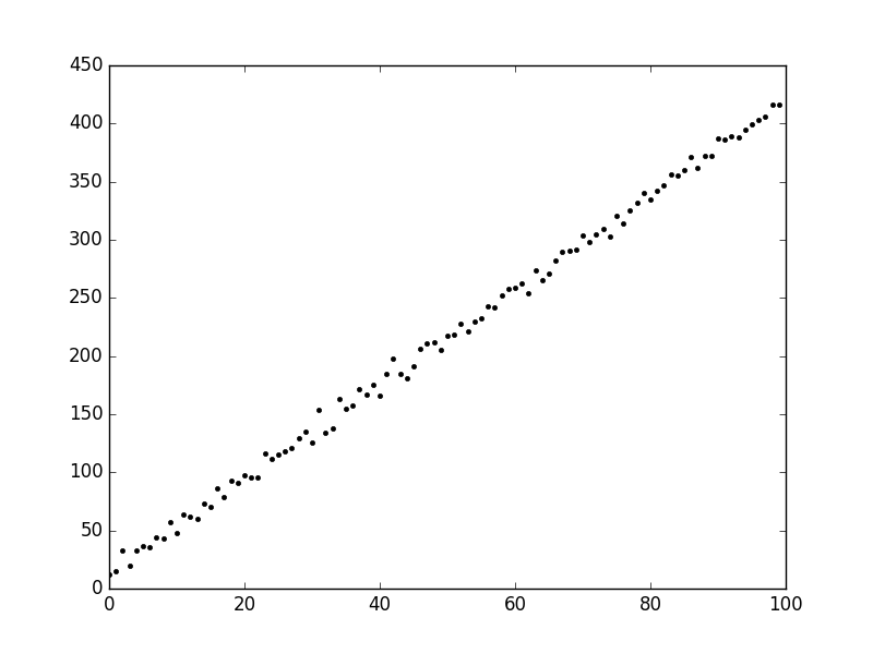
I generated this data myself with a linear equation. I also added some random noise to make it a little bit more realistic. Our goal will be to find a way to predict where a new data point will fall vertically given where it sits horizontally (in other words, the \(y\) value given the \(x\) value). We can state this goal as such:

Goal: Create a model that can reasonably predict new values based on the existing data

This is a pretty vague goal, and we’ll refine it as we progress.

You may remember from school something called the slope-intercept equation of a line. If you don’t here’s what it looks like:

Where \(x\) and \(y\) are the point coordinates, \(b\) is the \(y\)-intercept (where the line hits the \(y\)-axis), and \(m\) is the slope of the line.

We can rewrite this equation with some different symbols that are commonly used in machine learning like so:

The function \(h_\theta\) is called the hypothesis function, and it serves as our predictor. Given an \(x\) value, \(h_\theta(x)\) will produce what our model thinks \(y\) should be.

Using what we already have said about the slope-intercept equation, we can consider how we might be able to achieve our goal. We said that the \(\theta_0\) value determines the \(y\)-intercept of the line, or where it sits vertically. By increasing or decreasing \(\theta_0\), we can shift the line up or down, respectively. Additionally, \(\theta_1\) determines the slope of the line, or its angle. By modifying \(\theta_1\), we can tilt the line more or less. By combining these two mechanisms, shifting and tilting, we can create the line that resembles the data set.

\(\theta_0\) and \(\theta_1\) serve as the parameters of our model, since their values will directly determine how well our model can predict existing and new values.

(It should be noted that this is a relatively contrived and simple example with only two parameters, but the same principles apply even if we have more dimensions or even higher-order dimensions like \(x^2\) or \(x^3\).)

Now we can modify our goal slightly:

Goal: Find the values of the parameters, \(\theta_0\) and \(\theta_1\), that form a line that best “fits” our data.

But what do I mean when I say a line that “fits” the data? If we just look at a plot of our line on top of the data, we can get an intuitive feel of if the line is “good” or not. But what if our data has many dimensions and can’t easily be visualized? And how can we empirically determine which of two lines are better if they both seem pretty close to the data set?

To solve these problems, we’ll need a tool called the cost function. You may also see it called the error or loss function, but it all refers to the same concept. The cost function will let us “score” our model by determining mathematically how close or far it is from the original data. Many different cost functions exist, but most of them follow some scheme of measuring the distance between a model prediction (\(h_\theta(x)\)) and the actual value (\(y\)) for each data point.

For our example, we’ll use the sum of squares cost function, which is a common and effective cost function. To calculate the cost, we will loop over every data point, find the difference between the predicted and actual value, square it, then add up the result for all the data points. Mathematically, it looks like

We’ll also divide the sum by the number of data points, \(N\), which is called normalization. It allows our model’s cost to be independent of the number of the number of data points it was calculated against (i.e. adding more data doesn’t necessarily increase the cost). The division by 2 is somewhat arbitrary and not completely necessary. We do it to make some of the math in the future slightly cleaner.

With the cost function, we now have a way to actually evaluate how good (or rather, bad) our model is at predicting values. Ideally, we would want our parameters (\(\theta_0\) and \(\theta_1\)) to be such that the cost function is equal to 0, but that’s often impossible or even undesirable. So we’ll settle with minimizing the cost function to the lowest value we reasonably can, which means finding the parameter values that produce a lower cost than any other set of values. So let’s update our goal to reflect this new idea

Goal: Find the values of the parameters that forms the equation of a line that minimizes our cost function

Mathematically, this is called an optimization problem and can be written as such:

Optimization via Gradient Descent

Gradient descent is an algorithm that will allow us to perform the aforementioned optimization. The key insight to gradient descent comes from the shape of our cost function. If we plot out the cost function with some different values, we’ll likely get a “U” shaped curve like below.

This comes from the square term in our sum of squares function. Note that this graph is in two dimensions, where our actual graph of \(J(\theta_0, \theta_1)\) would be three-dimensional, but the same idea still applies.

So how can we determine a minimum from this curve? With gradient descent, we’ll pick an arbitrary set of starting values for our initial parameters (usually 0). The cost of those parameters will give us some point on the U curve of the cost function we were just looking at. Since we are aiming for the minimum, we’ll want to adjust our parameters such that the cost function will be less as a result. To figure out how to tweak the parameters to achieve this, we’ll take the derivative of the cost function, and subtract the current value of the parameter by that partial derivative (multiplied by a constant). We’ll then repeat this process over and over again, moving closer and closer to the minimum. Mathematically this can be described as

Repeat until convergence:
 for \(j = 0\dots m\):
  \(\theta_j := \theta_j - \alpha \frac{\partial}{\partial\theta_j}J(\theta_0, \theta_1)\)

A few things to note about this pseudocode

• “Until convergence” is user defined, but usually when the cost function stops decreasing by a significant amount after an iteration of the outer loop
• \(m\) is the number of parameters in the model
• \(\alpha\) is the learning rate, which will determine how big or little of changes to the parameters we make per iteration.
• Simultaneous update: we’ll have to calculate the new values of the parameters one at a time, but we want to update them all at once. We don’t want to mix new parameter values and old ones during the inner loop.

Intuitively, we can think of gradient descent as if we were trying to walk down a hill into a valley. The partial derivatives will tell us the “gradient”, or which direction we need to move in order to progress to the bottom. Each iteration of the outer loop is like taking a small step. Given enough steps, we’ll eventually make it to the valley floor, or the minimum of our cost function.

A nice debugging feature of gradient descent is that, when everything is working properly, the cost function should always decrease with every iteration. If the cost function stays the same, or only increases my an infinitesimal amount, then we’ve likely converged at the minimum. If it is ever increase, something has probably gone wrong and we should check our code (or adjust our learning rate to be smaller).

There’s one last thing we need to define before we can start implementing this algorithm in code, and that’s the partial derivative of the cost function. If you know multivariate calculus, feel free to try and derive this yourself, but for the sake of brevity I’ll simply give the answer below:

Where \(x_{n, j}\) is the \(j\)th feature value on the \(n\)th training set. Although we didn’t explicitly state it, we can think of each \(x\) example as a pair, \((1, x)\), that gets multiplied and summed to the respective parameter, \((\theta_0, \theta_1)\).

Naive Implementation in Python

Math is fun, but what does this all look like in code? For this example, I’m going to skip over the data collection and cleaning, and focus on the interesting parts. I’m going to assume that I have two (Python) lists, X and Y that hold the \(x\) and \(y\) values of our data set, respectively.

We’ll first break our X and Y lists into two separate sets of lists: X_train, Y_train, X_test, and Y_test. The rule of thumb for this split is about 70% of the examples will go to the training lists, and the other 30% will be reserved for testing.

Before we move any further, I want to stress how critical it is that we split up our data set into training and test sets. The training set will be used for the “learning” portion (determining the values of \(\theta_0\) and \(\theta_1\)), while the tests set will be used to evaluate how good of a model we have once the parameter values are set. The point here is that our ultimate goal is to have a model that’s general: it is effective at predicting new values that it hasn’t seen before. So if we try to test with the same data that we trained with, we have no idea if we’re achieving our goal, since all the test points will have been seen during training. With the segregated sets, we can determine if our model can be effective when it encounters new data.

The first thing we’ll need to do is define our hypothesis function. This is trivial since our simple model only has two parameters.

def hypothesis(theta0, theta1, x):
    return theta0 + (theta1 * x)

Next, we’ll need to define our cost function

def cost(theta0, theta1, X, Y):
    errors = [hypothesis(theta0, theta1, x) - y for (x, y) in zip(X, Y)]
    squared = [i * i for i in errors]
    return 1 / (2 * len(X)) * sum(squared)

Now we’ll define a descend function that will serve as one iteration of the gradient descent loop

def descend(t0, t1, X, Y):
    xy = zip(X, Y)
    N = len(X)

    # Calculate partial wrt theta0
    p0 = [hypothesis(t0, t1, x) - y for (x, y) in xy]
    p0 = (1 / N) * sum(p0)

    # Calculate partial wrt theta1
    p1 = [(hypothesis(t0, t1, x) - y) * x for (x, y) in xy]
    p1 = (1 / N) * sum(p1)

    new_t0 = t0 - LEARNING_RATE * p0
    new_t1 = t1 - LEARNING_RATE * p1
    return (new_t0, new_t1)

Finally, we’ll define our main function that will serve as the driver of the program

def main():
    # ...data generation omitted...
    theta0, theta1 = 0, 0
    old_cost = cost(theta0, theta1, X_train, Y_train)

    while True:
        theta0, theta1 = descend(theta0, theta1,
                                 X_train, Y_train)
        new_cost = cost(theta0, theta1, X_train, Y_train)

        # Check for convergence
        if abs(new_cost - old_cost) > EPSILON:
            break
        else:
            old_cost = new_cost

And that’s all we really need to implement linear regression with gradient descent. However, it may be useful to visualize the results and evaluate how good of a job we did. We’ll create some extra functions that let us do that.

def graph(t0, t1, X, Y):
    # using matplotlib.pyplot
    pyplot.plot(X, Y, color='r.')
    pyplot.plot(X, [hypothesis(t0, t1, x) for x in X])
    pyplot.show()

def r_squared(t0, t1, X, Y):
    Yp = [hypothesis(t0, t1, x) for y in Y]
    u = sum([(yp - yt)**2 for (yp, yt) in zip(Yp, Y)])
    mean = sum(Y) / len(Y_true)
    v = sum([(y - mean)**2 for y in Y])
    return (1 - (u / v))

The r_squared function implements a common statistical equation called \(R^2\). The details aren’t important; just know that a score closer to 1.0 is better.

scikit-learn Implementation

As painful as that might have been, luckily other people have done it before and given away their code for free. As a plus, they probably did it better.

scikit-learn (sklearn) is a popular Python library that’s full of handy algorithms for machine learning. Let’s take a look at how we can leverage this awesome resource for our example problem.

from sklearn.linear_model import LinearRegression
from numpy import array

# Transform X and Y to numpy vectors
X_train = array(X_train).reshape(-1, 1)
Y_train = array(Y_train).reshape(-1, 1)

# Perform the actual training
lr = LinearRegression()
lr.fit(X_train, Y_train)

# Predict and evaluate
y_15 = lr.predict(15)
r_squared = lr.score(X_test, Y_test) # must be vectors
params = lr.get_params()

And that’s it: the whole algorithm boils down to essentially two lines. You’ll note that we had to turn our lists into numpy vectors, and that is so that scikit-learn can do some internal optimization with our data to run faster.

Results

When I ran our implementation, I found that a learning rate of about 0.0003 worked well. Gradient descent took about 25,000 iterations to converge, but only about 2-3 seconds. We also got an \(R^2\) score of 0.9980. The results are plotted below.

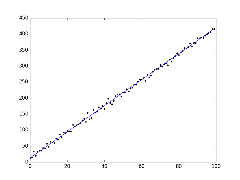
So even though our example was pretty simple, we did a pretty nice job fitting our data. Not bad for less than 50 lines of code!

Conclusion

Although this was a relatively simple example, these principles are foundational and used throughout machine learning. Indeed, machine learning can often seem magical (especially considering its powerful applications), but at the end of the day it boils down to some algorithms leveraging statistics quite nicely.

Here, we looked at one specific example of machine learning: linear regression with gradient descent. But tons of algorithms exists, like support vector machines, logistic regression, and artificial neural networks to name a few. Each has their own appeals and drawbacks that makes them more or less suited to particular problems.

Machine learning, and more broadly, artificial intelligence, can’t solve every problem. But they are an extremely powerful way of tackling problems that often seem impossible to accomplish through computation. We are still discovering new applications and methods for machine learning, and I have no doubt that it will even more of a dramatic impact on our daily lives in the near future.