What is deep learning?
Deep learning is a subfield of machine learning that has had remarkable research success in the past decade. Huge numbers of research groups and top software companies are pushing the boundaries of what was previously thought possible through computation with these advancements.
One of my favorite things about deep learning is that, despite the hype and number of PhD’s who work in the field, it is actually relatively simple to get started. Most common laptops are powerful enough to train and run simple deep models. This is in part due to the growing amount of open source machine learning libraries that make building deep models significantly simpler than rolling them by hand. In this post we’ll walk through some of the fundamentals of deep learning and the historical background. This foundations should provide enough context to start digging into deep learning and building your very own models.
Getting started
Deep learning is one specific category within the general field of artificial intelligence. At its core, it leverages learning models that are artificial neural networks with lots of layers. These models are general purpose, and similar architectures can be trained to run a variety of tasks. They “learn” by adjusting parameters, of which deep neural nets can have billions. We can think of these parameters as lots of dials on a big, complicated machine. By discovering the right combination of dial settings, we can configure the machine to properly accomplish a particular task.
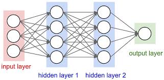
Neural networks are layers of groups of neurons that feed into each other. We’ll discuss more about the neurons in a moment, but suffice it to say that they perform a relatively simple mathematical transformation. Every neuron in a layer receives its input from every neuron in the layer before, and sends its output to every neuron in the next layer. There are three different kinds of layers in a typical network: input, hidden, and output. The input layer is the first layer in our network, and it is just the input for the task we’re trying to solve (e.g. each neuron corresponds to a pixel within an image). The output layer is what our model will ultimately result in for a given input. It may just be a single number or, if our model is dealing with multiple categories, it may be multiple outputs that we can combine in some meaningful way. Hidden layers are where all of the interesting things happen. They contain all the parameters in our model that are used during the mathematical transformation. By tuning the parameters in the hidden layer neurons, we train our network. Deep neural networks get their namesake by generally having lots of hidden layers.
A quick history of deep learning
Artificial neural networks were originally theorized in the late 1950’s and early 1960’s, and derive their name from the loose inspiration of how actual neurons within our brain work. Although the concept is almost as old as artificial intelligence itself, neural networks did not receive much attention until the 1980’s. By then, researchers discovered how to increase the size of these networks without dramatically increasing the training complexity. However, they again fell out of vogue due to their inability (at the time) to outperform other machine learning algorithms.
All of this changed in 2006, when deep learning was born. Huge advancements in computer hardware and some algorithmic improvements permitted researchers to build neural networks with huge numbers of layers (i.e. “deep”) and train them to beat other kinds of machine learning models. This marked the start of the era of deep learning, where these models have been adapted and modified to perform amazingly well in a wide variety of complex tasks. Many times, they can even outperform humans.
Going deeper: What’s in a neuron?
Neurons within a deep learning network perform a mathematical transformation of their input that is determined by some parameters, or weights. There’s a lot of variety within the general model, but most models do a linear combination of their weights and the input (easily calculated by a matrix-vector multiplication), followed by some nonlinear “activation function”. The activation function is important to make our models learn nonlinear data, and several kinds exist. In equation form, we can describe what happens within a neuron by
\[h = \sigma(x_1\theta_1 + x_2\theta_2 + \cdots + x_n\theta_n)\]where \(x_n\) is the input, \(\theta_n\) are the weights, and \(\sigma()\) is the activation functions. The most popular activation functions, called rectified linear unit (ReLU), defined as \(\sigma(z) = \text{max}(0, z)\).
Training a neural network: Optimization and backpropagation
By tuning the model parameters, we can teach our neural network to perform a task. But how do we know how to adjust those parameters? This is particularly difficult in deep models that are complex and have parameters on the order of billions.
The way most deep models are trained follows an optimization procedure. When a model produces a result, we can define an error function (also known as a cost function) that measures how incorrect our model is. Then we can define the training procedure as an optimization problem: we want to find the model parameters such that the error on our training set is minimized.
To actually perform this minimization, most deep learning models make use of an optimization algorithm known as stochastic gradient descent (SGD). This algorithm repeatedly approximates the gradient of the error function, and then slightly moves the parameters in the direction that will decrease the error. The gradient can be calculated through a procedure known as backpropagation. Essentially, the gradient gives us an idea of how much blame to assign to ever parameter in our network for a prediction. By calculating the blame for a number of inputs, we can approximate how the parameters are affecting the model’s accuracy generally. Then, we can adjust the parameters such that they will hopefully make our model more accurate. By repeating this enough times, we can train our neural network by tuning all the parameters.
Deep learning variations
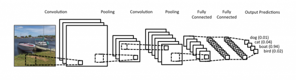
Vanilla neural networks can be useful, but we can get even better results if we modify the model to utilize some inherit characteristics of our objective task. For instance, within images, the pixel data often has a high spatial dependence, meaning that pixels close together often work together to make out specific attributes within an image. We can exploit this fact by utilizing a convolutional neural network. Without getting into the details, convolutional neural networks (also known as convnets) replace some of the early layers with neurons that perform a convolutional operation. This combines areas of a picture using math and lets us extract spatial information from our inputs.
Another variation of the typical (or feedforward) neural network involves making use of temporal dependencies, or when the correct output depends on multiple inputs spaced out over time. Temporal dependencies are really common, for instance speech recognition and text comprehension. To exploit these dependencies, models known as recurrent neural networks (RNNs) are typically used. These are neural networks where some of the neurons feed back into previous layers, creating a cycle. When inputs are sequentially fed into the network, part of the calculations will depend on not only what the network currently sees, but what it has previously seen. The mechanisms for when and how to feed back into the network can get pretty advanced, and can even mimic our understanding of how our own brains work, such as the long short-term memory (LSTM) neuron.
Deep learning has also significantly improved other areas of machine learning. A great example of this is within reinforcement learning, where models are “agents” that try to perform a specific task like win a game against an opponent or traverse a robot through a maze. Although the algorithms required to perform reinforcement learning don’t necessitate deep neural networks, they have benefited from the accuracy and generalization abilities of these models. For instance, most of the interesting problems in reinforcement learning have a huge search space, meaning that the number of possible states (e.g. chess positions, robotic sensor data) the agent could be in is enormous and impossible to completely exhaust during training. However, the agent will still need to take actions in these states, even though it has not seen them before. To solve this, we can represent the state space with a deep neural network, which can learn what “kind of” state its in, and approximate it feasibly for the agent. Other calculations the agent performs can be similarly approximated. Because deep networks generalize so well (meaning they give similar outputs for similar, though distinct, inputs), the agent can encounter entirely novel situations and still act appropriately because it has learned what to do in similar states.
Conclusion
Deep learning has moved the field of machine learning and artificial intelligence dramatically forward and into the forefront of our technological future. However, despite all the hype, it turns out that deep learning is really some manageable mathematics and algorithms, refined and improved over a half century or so. Ultimately, the models will keep improving and expanding their capabilities beyond even what we’ve seen so far. Now is an amazing time to jump in on deep learning, to both discover more about the nature of intelligence and leverage our existing knowledge to improve the world we live in.