Getting Started with Tensorflow
Note: All the code from this post can be found here. This tutorial is adopted from Google’s own TensorFlow tutorial, “Deep MNIST for ML Experts”
My last post talked about deep learning very generally, describing the fundamentals of how deep neural networks work and are used. In this post, we’ll look more concretely at actually building a convolutional neural network to classify handwritten digits from the MNIST data set. Using Google’s popular machine learning library TensorFlow, we’ll have a model that gets over 98% accuracy with about 150 lines of code and 10 minutes of training time on my laptop.
Prerequisites
This tutorial assumes that the reader has a basic familiarity of programming in Python. If you’ve never seen the syntax before, it is pretty easy to pick up. I also assume that you have TensorFlow installed on you machine. For the sake of brevity, much of the fundamentals of deep learning are omitted, but you can learn about those in my previous blog post.
What is TensorFlow?
TensorFlow is a high performance numerical computing library developed by Google. It generally supports any kind of scientific computation, but was developed specifically with machine learning in mind. TensorFlow has lots of packages that make building and running deep and even distributed neural networks much simpler than before. It was open sourced by Google in 2015.
Before TensorFlow’s arrival, many of the machine learning libraries in use were developed by research labs to support their needs. While these libraries were great, they often lacked strong software engineering expertise and failed to meet enterprise scale needs. Thankfully, TensorFlow was developed from the ground up by experts in both of these domains. TensorFlow is the product of choice that Google, a machine learning leader, uses in many of their products.
Another great aspect of TensorFlow is that the models are portable. A TensorFlow program trained to run on a rack of servers can be deployed to execute on a smartphone. As we will discuss in a moment, this is because TensorFlow builds computational graphs that can be stored independently of the program that developed them. The parameters can be trained, and then the model shipped off to run in production. TensorFlow can also utilize specialized hardware like graphics processors without any explicit programming by the end user.
Programming in TensorFlow
TensorFlow was originally developed in C++, but language bindings for Python are the most common way people program their machine learning applications. TensorFlow operates by building a computational graph that can be executed. This differs slightly from typical imperative programming, where each statement is explicitly executed line by line. Instead, TensorFlow has us describe how to make certain calculations, and then when we want, we can evaluate them against a session, feeding in any potential inputs. Let’s look at an example
import tensorflow as tf
sess = tf.Session()

x = tf.placeholder(tf.float32)
y = x * x
z = y + 100

sess.run(z, feed_dict={x:42})

# >>> 1864.0
First, we defined x as a placeholder: this is essentially an input to our
computational graph. Then we told TensorFlow how to calculate y and z.
Finally, we told TensorFlow to actually calculate the value of z, populating
the value for our placeholder x.
This was a pretty simple example, but it illustrates the basic mechanics of programming in TensorFlow. However, let’s add some complexity. TensorFlow derives its name from the tensor: a mathematical generalization of a matrix. Tensors are kind of like arbitrarily high-dimensional arrays, and TensorFlow excels at working with these constructs. For instance, if we have 100 images, each 28 by 28 pixels in size, with three values for the red, green, and blue, we can represent all that data as a single 100x28x28x3 tensor. Let’s try an example of programming with tensors through matrix-vector multiplication.
# Matrix-vector multiplication
A = tf.placeholder(tf.float32,
                   shape=[3, 3])
b = tf.placeholder(tf.float32,
                    shape=[3, 1])
z = tf.matmul(x, y)

sess.run(z, feed_dict={
  A:[[1, 2, 3], [4, 5, 6], [7, 8, 9]],
  b:[[1], [2], [3]]
})

# >>> [[14.],[32.],[50.]]
TensorFlow has lots optimized implementations of common operations like
matmul. These are really helpful when building deep neural networks that are
blazingly fast.
Before we start building a deep neural network, we need to introduce the idea of
TensorFlow variables. Variables are dynamic values that are global to a
TensorFlow session. Generally these are used as the parameters in models that
are tuned during training. Although we won’t directly manipulate them, the
optimization procedure that we utilize will. Before we can start using our
variables in a session, though, we will need to execute
sess.run(tf.global_variables_initializer()) in our program.
Building an MNIST classifier
Now let’s get started building an MNIST image classifier. The MNIST is a common data set of 28x28 pixel images of handwritten digits. They were scraped from tax forms, then centered on the image.
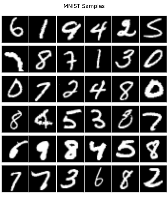
The goal of our model is to input these images as arrays of pixels and learn how to derive which digit is displayed in the image. This is called classification, since each image has to fall within 10 categories (the number 0 to 9).
To accomplish this feat, we’re going to utilize a deep convolutional neural network. We’ll have a total of 4 layers: the first two convolutional, the last two fully connected. To prevent overfitting, we’ll utilize dropout. And finally, our outputs will be converted into a probability distribution via the softmax functions. It’s not necessary that you fully understand all the details; these are just common practices within deep machine learning.
To get started, we’re going to build some helper methods that will make constructing our model a little less tedious. The code presented in this tutorial will be somewhat out of order, but it should run fine when combine (remember, all of the code in this tutorial can be found here, with some additional features).
# Create some random variable weights
def weights(shape):
  return tf.Variable(tf.truncated_normal(
      shape, stddev=0.1))

# Create a “constant” bias variable
def bias(shape):
  return tf.Variable(tf.constant(
      0.1, shape=shape))

# Hardcode our convolution parameters
def conv2d(x, W):
  return tf.nn.conv2d(x, W,
      strides=[1, 1, 1, 1], padding='SAME')

# Same with our maxpooling
def max_pool(x):
  return tf.nn.max_pool(
      x,
      ksize=[1, 2, 2, 1],
      strides=[1, 2, 2, 1],
      padding='SAME'
    )
The first two methods define the initialization for weights and constants that we’ll use in our model. The last two methods hardcode some of our parameters for our convolutional operations.
Next, we’ll actually define our model. We will encapsulate it as a method so as to keep our main method a bit cleaner. The model will take a tensor input for an argument and return it’s output predictions (as well as the dropout probability used, though that’s not significant).
def cnn(x):
  keep_prob = tf.placeholder(tf.float32)
  imgs = tf.reshape(x, [-1, 28, 28, 1])

  # Layer 1
  W_conv1 = weights([5, 5, 1, 32])
  b_conv1 = bias([32])

  z_conv1 = conv2d(imgs, W_conv1) + b_con1
  h_conv1 = tf.nn.relu(z_conv1)
  h_pool1 = max_pool(h_conv1)

  # Layer 2 (convolutional)
  W_conv2 = weights([5, 5, 32, 64])
  b_conv2 = bias([64])

  z_conv2 = conv2d(h_pool1, W_conv2) + b_conv2
  h_conv2 = tf.nn.relu(z_conv2)
  h_pool2 = max_pool(h_conv2)

  # Layer 3 (fully connected)
  W_fc1 = weights([7*7*64, 1024])
  b_fc1 = bias([1024])

  h_pool2_flat = tf.reshape(h_pool2, [-1, 7*7*64])

  z_fc1 = tf.matmul(h_pool2_flat, W_fc1) + b_fc1
  h_fc1 = tf.nn.relu(z_fc1)
  h_fc1_drop = tf.nn.dropout(h_fc1, keep_prob)

  # Layer 4 (fully connected, last hidden layer)
  W_fc2 = weights([1024, 10])
  b_fc2 = bias([10])

  z_fc2 = tf.matmul(h_fc1_drop, W_fc2) + b_fc2
  h_fc2 = tf.nn.relu(z_fc1)

  return h_fc2, keep_prob
For each layer, we define our weights and biases (TensorFlow won’t reinitialize these during execution), and perform our operation before moving on to the next layer. For the convolutional layers, this involves applying the actual convolution followed by a maxpooling to decrease the dimensionality. For the fully connected layers, the operation is a matrix vector multiplication with the weights, followed by an ReLU activation (and dropout in the second to last layer). When switching from convolutional to fully connected layers, we needed to reshape our data.
Now that our model has been established, we can program our training procedure. When training a deep neural network, we typically feed in some data, measure the error, and adjust the parameters so as to decrease the error. Our input data and labels will be placeholders, and we can measure the error using TensorFlow’s built-in cross entropy operation on the softmax of our model outputs. Then we can program that our optimization step (i.e. weight adjustment) should use the Adam optimizer, which is an enhancement of stochastic gradient descent. While we’re at it, we’ll also tell TensorFlow how to measure our accuracy.
def main(_):
  mnist = input_data.read_data_sets(
    FLAGS.data_dir, one_hot=True)

  x = tf.placeholder(tf.float32,
                     [None, 784])
  y_true = tf.placeholder(tf.float32,
                               [None, 10])
  y_hat, keep_prob = cnn(x)

	# Cross entropy measures the error in our predictions
  cross_entropy = tf.reduce_mean(
    tf.nn.softmax_cross_entropy_with_logits(
      logits=y_hat, labels=y_true))
  # Once we have error, we can optimize
  training_step = tf.train.AdamOptimizer(1e-4).minimize(cross_entropy)

  # Define a “correct prediction” to calc accuracy
  correct_prediction = tf.equal(tf.argmax(y_hat, 1),
      tf.argmax(y_true, 1)
  accuracy = tf.reduce_mean(tf.cast(correct_prediction, tf.float32))
Now we can write the actual loop that will run the training procedure.
  # inside main()
  with tf.Session() as sess:
    sess.run(tf.global_variables_initializer())
    for i in range(EPOCHS):
      batch = mnist.train.next_batch(MINIBATCH_SIZE)
      train_step.run(feed_dict={
        x:batch[0],
        y_true:batch[1],
        keep_prob:0.5
      })

  test_acc = accuracy.eval(feed_dict={
    x:mnist.test.images,
    Y_true:mnist.test.labels,
    keep_prob:1.0
  })

  print('Test accuracy is {:2f}%'.format(test_acc * 100))
Finally, we can put the finishing touches so that our program will run. Outside of any function, at the bottom of the file write:
from tensorflow.examples.tutorials.mnist import input_data
import tensorflow as tf

if __name__ == '__main__':
  EPOCHS = 5000
  MINIBATCH_SIZE = 50

  tf.app.run(main=main)
On my 2013 MacBook Pro, I was able to run this program in about 5-10 minutes, and achieved 98% accuracy. That’s pretty amazing! All of this code, including some enhancements like model saving, can be found at this link.