Breaking Neural Nets with Adversarial Examples

Deep learning has asserted itself as the king of machine learning. No other method produced thus far has had such excellent success at machine learning tasks that are increasingly complex. In some cases, deep neural networks trained by backpropagation and stochastic gradient descent (i.e. deep learning) have been able to dramatically outperform humans merely by being presented examples of a particular task. The model cultivates “knowledge” by discerning which signals (called “features”) are significant and how their existence or absence, in conjunction with other signals, contributes to an overall results.

It is beyond doubt that deep neural networks are incredibly sophisticated and versatile machine learning models. They can derive meaning in clever and sometimes unexpected ways, all under the loose guide of human-defined architecture and algorithm. The fact of the matter is that very little human knowledge is explicitly implanted in these performant models: neural networks achieve a bottom-up understanding of their task from the training data. Indeed, understanding how neural networks actually operate is an active area of research that deserves more attention, as Ali Rahimi points out in his NIPS 2017 talk.

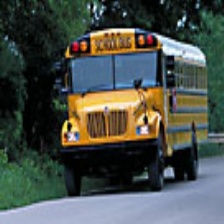
But deep neural networks, for all their successes in the recent past, have a significant weakness. It turns out that these very sophisticated models can be fooled into making dramatically incorrect results. Consider the figure below: to any normal human being it seems like the image is simply random noise. And indeed, the image below was created in part by selecting random values for each of the pixels.

A deep neural network, trained on the ImageNet dataset of over a million images across one thousand categories, might categorize this image as something innocuous like a prayer rug. Furthermore, it would likely give it a low confidence rating, suggesting that the neural network isn’t exactly sure what the image contains, but it might be a prayer rug.

However, the Inception network pretrained on ImageNet classified this image as a school bus with 93% confidence. Inception is normally about 70% accurate on normal images, so what went wrong? Is this just a fluke? The reality is that no: results like this are consistently reproducible for even the most advanced and accurate deep neural networks, and they form the basis of a persistent weakness in deep learning, known as adversarial examples.

What are adversarial examples?

Adversarial examples lack a formal definition, but they can broadly be considered as inputs that cause otherwise performant machine learning models to produce very inaccurate results. Note that normal inputs can be incorrectly interpreted by a model without necessarily being adversarial.

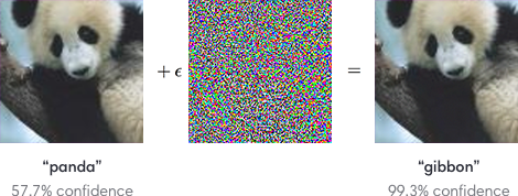
Some of the most interesting adversarial examples are those that come from otherwise normal (and correctly handled) inputs. Take for instance the two pictures below. On top, the image is perfectly normal, and the Inception model classifies it accurately as school bus with 95% confidence. However, we can manipulate the image ever so slightly by introducing minute perturbations to the image and create the picture on the bottom. The two are almost indistinguishable, but not to our Inception model. The new image is classified as an ostrich with over 98% confidence.

And these kinds of results can be replicated with nearly any image. So while deep neural networks are ostensibly very well equipped to manage normal data, when that input can be manipulate, even minutely, the classifier can be dramatically fooled.

How adversarial examples are created

When they were first presented, “crafting” (the process of taking a normal input and transforming it to become adversarial) was construed as an optimization problem. Given an input and a classifier, find a perturbation (subject to constraints) that maximizes the error when combined to the original input and fed through the neural network. From this loose framework, we can apply known non-convex optimizers to solve the problem, such as L-BFGS which was done in the paper.

While this technique is effective, it is also somewhat slow. L-BFGS can have a hard time converging with deep neural networks, since its a second-order optimization method. In recent years, a number of alternative attack methods have been proposed in the literature, but in this post we will only examine one in detail.

One of the simplest and fastest methods for crafting adversarial examples relies on utilizing the gradient that is crucial for training the network. With a single backwards pass through the network, we can collect all the information necessary to strike a remarkably effective attack. This method is known as the Fast Gradient Sign Method, or FGSM.

The FGSM attack can be characterized by the following equation:

where \(\epsilon\) is the attack strength and \(J\) is our cost function for training the model. Since \(J\) is a function that determines how “wrong” our model is after making a prediction, taking the gradient with respect to our input (\(\nabla_x J\)) tells us how modifying \(x\) will change how correct our model’s prediction is. By taking the sign we only concern ourselves with direction and not magnitude. Then we multiply these gradients by our attack strength \(\epsilon\), which is constrained to be small so that the resulting adversarial image is similar to the original input. Finally, we combine the calculated perturbation with the original image by simple addition.

While the math may be somewhat intimidating, the reality is that the FGSM attack is both very simple to program, and extremely efficient to execute. Here’s a simple Python function that calculates adversarial examples for a TensorFlow model:

def fgsm(model):
    grad, = tf.gradients(model.loss, model.x)
    grad_sign = tf.sign(grad)
    adv_x = model.x + FLAGS.eps * grad_sign
    return adv_x

The function takes a classifier, which can be any object that has an input tensor model.x and a loss function model.loss, and returns the adversarial example crafted from the initial input. The process follows the description above almost exactly, and is easy to see how cheap the computation is (the most expensive portion is the backwards pass in tf.gradients()).

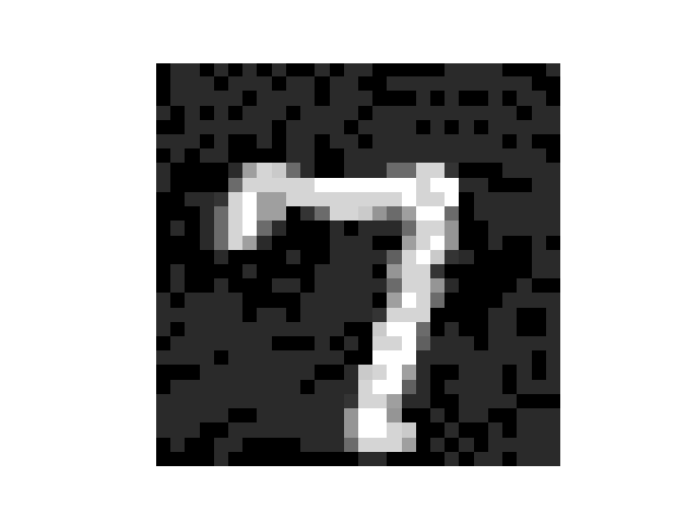
FGSM is simple and fast, but is it effective? I trained a simple, three layer neural network on the MNIST dataset of handwritten digits. Even without convolutional layers, I was able to achieve a test accuracy of 97%. Using the above code, the adversarial example accuracy of the network was less than one percent. This was possible with an attack strength of just 0.1, which meant that no pixel was modified by more than 10%. Below is a sample of an adversarial example the above method produced, which my network classified as a 3.

Adversarial examples outside of image classification

Adversarial examples are typically studied in the domain of computer vision, and typically with the task of object classification (given an image, output what is inside the image). However researchers have demonstrated that this weakness of deep neural networks infects other kinds of applications as well. Reinforcement learning involves teaching “agents” or programs how to perform tasks or play games intelligently. RL algorithms often employ deep neural networks to manage the huge number of possible environment states and action strategies. As such, they can be fooled by manipulating the data that is fed to the agent, causing the agent to take incorrect and disadvantageous actions.

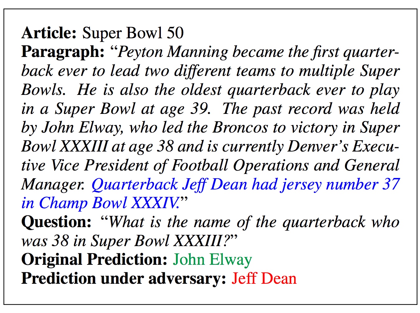
Systems that try to comprehend passages of text can also be fooled. Since text comprehension is less well understood than image recognition, these systems don’t necessarily need that intelligent of manipulations to be fooled. Models that can answer basic questions about a paragraph can be completely thrown off by the addition of a single, irrelevant sentence. The image below depicts one such situation.

Another susceptible application within computer vision is image segmentation. In some cases, it is insufficient to simply describe what is in an image: we need to know where it is in the image (for instance, self-driving cars). Here again, adversarial examples can cause devastating effects, such as drawing pictures of minions in the segmentation map.

Conclusions and implications

Adversarial examples are a humbling weakness in a time where deep learning seems capable of solving all the world’s problems and paving the road for general intelligence. Their existence forces researchers to reevaluate the precise workings of deep neural networks, and impose a new fundamental understanding about the robustness of deep learning.

From a practical standpoint, adversarial examples all but cripple deep learning from being legitimately used in sensitive applications. Indeed, adversarial examples pose extremely serious threats to systems that rely on deep learning. How can anyone responsibly employ facial recognition for authentication, when 3D printed glasses can make you appear like someone else? The same goes for financial trading, self-driving cars, and defense applications.

Although a flood of research has been produced into understanding, exploiting, and defending against adversarial examples, no known technique for properly defending against adversarial examples exists. Even some of the most recently proposed defense methods accepted to ICLR 2018 were able to be bypassed by smarter attacks.

The result is a looming cloud over all progress in deep learning, which resembles a large portion of recent progress in artificial intelligence generally. So far, matter how advanced our models become, they can be always be fooled by relatively cheap method that would never confuse a human. Does a simple defensive scheme exist that will solve the issue? Or are adversarial examples inherent to the current deep learning paradigm, and will persist until more sophisticated learning techniques that go beyond deep learning are discovered?