Mastering the Learning Rate to Speed Up Deep Learning
Efficiently training deep neural networks can often be an art as much as a science. Industry-grade libraries like PyTorch and TensorFlow have rapidly increased the speed with which efficient deep learning code can be written, but there are still a lot of work required to create a performant model.
Let’s say, for example, you want to build an image classifier model. A convolutional neural network would be the proper approach to utilize deep learning. But how many layers go in your network? How much momentum and weight decay should you use? What’s the best dropout probability?
The reality is that these questions don’t have definitive answers. What works great on one dataset might not work nearly as well on another. There are sensible defaults and good rules of thumb, but finding the best combination is nontrivial. These kinds of decisions are known as hyperparameters: values that are determined prior to actually executing the training algorithm. Figuring out the optimal set of hyperparameters can be one of the most time consuming portions of creating a machine learning model, and that’s particularly true in deep learning.
Difficulties in Finding the Right Hyperparameters
Unlike the parameters inside the model, the hyperparameters are difficult to optimize. While it’s possible to optimize hyperparameters with Bayesian methods, this is almost never done in practice. Instead, the best set of hyperparameters is typically sought through a brute force search.
Part of the difficulty of finding the right hyperparameter values is their complex interplay between each other. One value of weight decay may work well for a particular learning rate and poorly for another. Changing one value impacts many others in ways that are difficult to control.
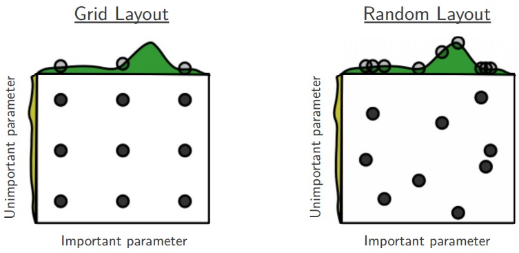
A tempting, naive method is to set up reasonable steps for each hyperparameter, and loop over a range, trying different values for each one. This is known as grid search, and it’s generally a bad idea for two reasons. First, the model has to be completely retrained for each set of hyperparameters, and the number of sets grows exponentially with the number of hyperparameters. Most of these values will be suboptimal, meaning that we’re wasting a great deal of time and energy unnecessarily retraining out model. The second reason is a little more subtle. Our steps will need to have a reasonable size to reduce the number of times we need to retrain the model, meaning we’re jumping over a decent bit of the search space with each iteration. There’s no reason our particular intervals are likely to contain good values, so it very possible we will entirely skip over good values. In fact, just doing a random search will usually yield better results that stepping across a fixed interval. The picture below depicts this visually.
Unfortunately, the state of the art in hyperparameter selection is little more than a random search. Most values have sensible defaults, but picking the best possible set can have a significant impact on the model’s final performance. Many machine learning researchers and practitioners develop intuitions about good values and how hyperparameters interact, but it takes a lot of time and practice. However, some recent and exciting research has outlined techniques for finding arguable the most important hyperparameter: the learning rate.
What is the Learning Rate?
Neural network training is typically performed as stochastic optimization. We start out with a random set of network parameters, find out which direction they should move to be improved, then take a step in that direction. This process is known as gradient descent (the stochastic portion comes from the fact that we find our improvement direction on a random subset of the training data). The learning rate determines how big of a step we take in updating the parameters.
# w is our weight, and dw is the derivative
w += -learning_rate * dw
The above parameter update occurs every iteration of the training process (though modern networks almost always use a more sophisticated update that adds extra terms). Without a doubt, the learning rate is the single most important hyperparameter for a deep neural network. If the learning rate is too small, the parameters will only change in tiny ways, and the model will take too long to converge. On the other hand, if the learning rate is too large, the parameters could jump over low spaces of the loss function, and the network may never converge.
3e-4 is the best learning rate for Adam, hands down.
— Andrej Karpathy (@karpathy) November 24, 2016
Picking the learning rate is pretty arbitrary. There are a range of reasonable values, but that range and the optimal value will vary with the architecture and dataset. As Andrej Karpathy joked in a tweet seen above, saying that one learning rate is “the best” is pretty preposterous.
Commonly, the ideal learning rate will change during training. Most world-class deep architectures are trained with a piecewise annealing strategy: train the network for a while with one learning rate, and when the model stops improving, decrease the learning rate by some factor and keep going. Intuitively, this makes some sense: if the model gets to a low spot in the loss space, the steps we take may be too big to keep from jumping across deeper valleys. Decreasing the learning rate allows for a more fine-grained training.
While piecewise annealing works in practice, we’ll soon see that it is suboptimal. There are better ways that we can (1) systematically find appropriate learning rate(s) for our particular problem, and (2) schedule the learning rate to automatically vary for faster training and improved performance.
Cyclical Learning Rates
Picking the perfect learning rate is hard. In fact, it’s probably too hard to find the singular best value. Instead, we can pick a range of learning rates and move through them during training. Kind of surprisingly, this method of cyclical learning rates works pretty well.
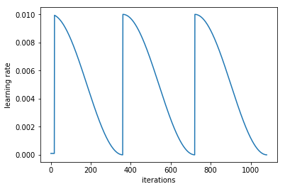
Cycling through values for the learning rate during training alleviates two of the problems with picking the learning rate. First, we don’t need to find an exactly perfect value, just a range of potentially good values. If we pick our range well (more on that shortly), we will be close to the optimal value for most of the training cycle, which is much better than randomly searching for the perfect learning rate. Additionally, we no longer need to manually schedule the learning rate to decrease during training, since the cycle does it for us. Just be sure to start the cycle with a high rate, and decrease it to a low rate.
You might be asking yourself why immediately reset the learning rate to a high value instead of allowing it to gradually climb back up. Resetting to a high learning rate gives us the benefit of a warm restart in our optimization and can improve our generalization. Remember that in machine learning, our primary goal is not to create a model that works well on the training data, but has high performance on the test data. This means that we not only want to find a low spot in the loss space during training, but we also want a very wide space. That way, even when our model is presented with new data that moves it around in loss space, it’s still likely to be at very low spot, and hence very accurate. Warm restarts helps us find those low and wide spaces that we’re looking for. Even if we find a cozy low valley with our low learning rate, restarting it to a high value at the start of a new cycle will pop us right out of that space if it’s not wide enough.
There are several ways to tinker with cyclical learning rates that might improve the final results. The length of a cycle is usually about an epoch, but longer cycles are possible. We can even increase the length of the cycle after each cycle. For instance, start with a cycle length of one epoch, then two epochs, then four, and so on. Schedules like this often give good results in part because they spend more time at lower rates during the end of training, allowing the model to hone in on an optimal space of the loss.
Cyclical learning rates allow us to circumvent the difficulty of picking a good learning rate. All we need are approximate bounds, and we can spend the majority of our training time being close to the optimal value, even as that optimal value changes during training. Additionally, we get the added benefit of restarts that will help us find wide areas in the loss space, improving our generalization ability. Now all we need is a method to find the approximate bounds to cycle through.
The LR Range Test
Cyclical learning rates preclude us from needing to find an optimal learning rate, but we still need an upper and lower bound for our cycles. Luckily, we don’t need to resort to the guessing game and random search that plagued or initial hyperparameter search. Instead, the paper that described the cyclical learning rate method also introduced a systematic method for finding good boundaries: the LR Range Test.
The LR Range Test is simple to understand and cheap to execute. Start with your initialized network, and pick a very small learning rate (much smaller than you would ever likely use). As you train, exponentially increase the learning rate. Keep track of the loss function for each value of the learning rate. If you’re in the right range, the loss should drop, then increase as the learning rate gets too high. Below is a graph of the loss value as a function of the learning rate.
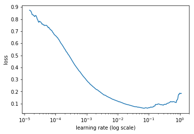
Looking at a plot of the loss vs. the learning rate, we can find our boundaries to use for our cycles. The place to look for is the learning rate where the loss stops decreasing: the minimum value. In the graph above it’s roughly \(10^{-1}\). This value is probably too high to use as our boundary, which is why the loss stopped decreasing here. We need to go back just a bit to a smaller value for our maximum boundary to use in our cycles. A good one to use here would be \(10^{-2}\). At that point the loss is still decreasing with some gusto. We wouldn’t want to pick the value with the steepest slope, since this will be the maximum, and the cycle will only spend a little while at that point. For the minimum, we can use any value that is smaller; typically we can divide the maximum by a factor such as 3 or 10.
Pedal to the Metal: Super-Convergence
Cyclical learning rates work well in practice, but there’s actually a way to take it a step further. The technique was introduced by Leslie Smith again and dubbed super-convergence. This strategy is a modification of the cyclical learning rate, and allows for training to converge substantially faster, hence the name.
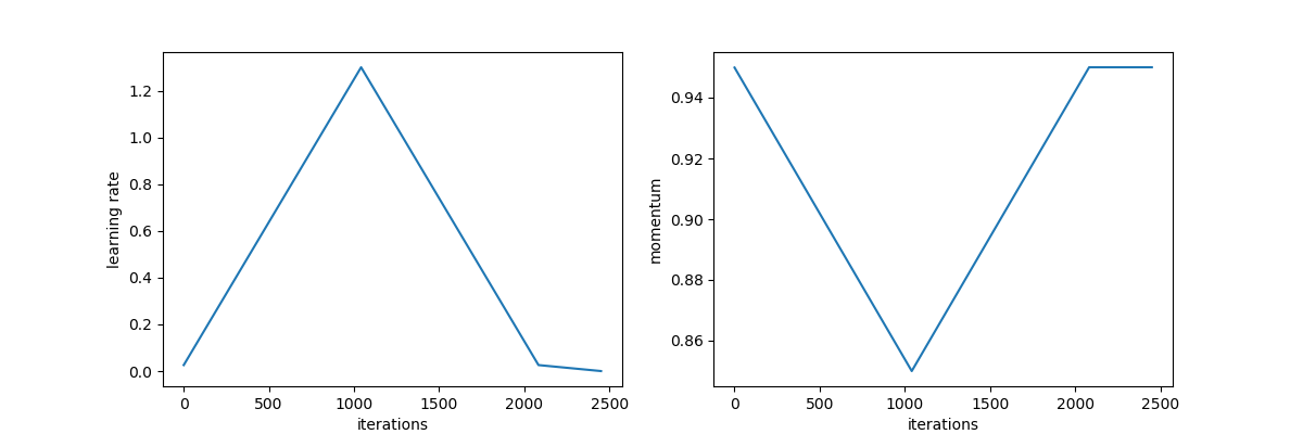
To exploit super-convergence, instead of iterating over cycles of the learning rate, we use a single “1cycle” policy. We derive the maximum and minimum learning rate from the LR Range Test as before. Now, we take one long cycle, moving up from the minimum to the maximum, and back down again. Then we continue training and decreasing the learning rate. We also inversely cycle the momentum, going from a high to low, and allowing it to continue increasing. A plot of the learning rate and momentum schedules are shown below.
Amazingly, adopting the 1cycle policy permits incredibly fast training. The original authors reported training deep networks on large datasets in a fraction of the epochs required by other training regimes. Recently, fast.ai leveraged super-convergence to train an ImageNet model in less than three hours, and a CIFAR10 model in lest than three minutes.
Conclusion
There are many difficulties in training deep neural networks. The best practitioners have spent a long time cutting their teeth and developing intuitions about the best values for hyperparameters. Fortunately, research has shown us better ways to pick the learning rate than wasting time and computing power fumbling around in the dark. The LR Range Test provides a quick way to find suitable boundaries for the learning rate, which we can cycle through during training to completely avoid having to find an optimal value. This means more time can be spent training more networks, and less time searching for hyperparameters. Additionally, the 1cycle policy lets us train neural nets at breakneck speeds, creating performant models in a fraction of the training time.
Special thanks to the fast.ai course for providing the inspiration and instruction for this blog post.