Building a World-Class CIFAR-10 Model From Scratch
In this post, I walk through how to build and train a world-class deep learning image recognition model. Deep learning models tout amazing results in competitions, but it can be difficult to go from a dense, technical research paper to actually working code. Here I take one of those papers, break down the import steps, and translate the words on the page into code you can run and get near state-of-the-art results on a popular image recognition benchmark.
The problem we will be solving is one of the most common in deep learning: image recognition. Here, our model is presented with an image (typically raw pixel values) and is tasked with outputting the object inside that image from a set of possible classes.
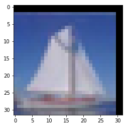
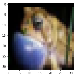
The dataset will be using is CIFAR-10, which is one of the most popular datasets in current deep learning research. CIFAR-10 is a collection of 60,000 images, each one containing one of 10 potential classes. These images are tiny: just 32x32 pixels (for reference, an HDTV will have over a thousand pixels in width and height). This means the resulting images are grainy and it’s potentially difficult to determine exactly what’s in them, even for a human. A few examples are depicted below.


The training set consists of 50,000 images, and the remaining 10,000 are used for evaluating models. At the time of this writing, the best reported model is 97.69% accurate on the test set. The model we will create here won’t be quite as accurate, but still very impressive.
The architecture we will use is a variation of residual networks known as a wide residual network. We’ll use PyTorch as our deep learning library, and automate some of the data loading and processing with the Fast.ai library. But first, let’s dig into the architecture of ResNets and the particular variant we’re interested in.
The Residual Network
Deep neural networks function as a stack of layers. The input moves from one layer, to the next, with some kind of transformation (e.g. convolution) followed by a non-linear activation function (e.g. ReLU). With the exception of RNNs, this process of pushing inputs directly through the network one layer at a time was standard practice in top-performing deep neural networks.
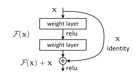
Then, in 2015, Kaiming He and his colleagues at Microsoft Research introduced the Residual Network architecture. In a residual network (resnet, for short), activations are able to “skip” past layers at certain points and be summed up with the activations of the layers it skipped. These skip connections form what are typically referred to as a residual block. The image below depicts one block in a resnet.

Architectures built by stacking together residual blocks (i.e. resnets) train much more efficiently and to less error. The original paper explores various depths, and are able to train networks of over 1,200 layers. Before, it was difficult to train networks with just 19 layers. One potential reason resnets allow for deeper networks is because they allow the gradient signal from backpropagation to travel further back up through the network, using the skip connections like a highway to get closer to the input layer. In 2015, a residual network won the ImageNet with 3.57% test error.
The authors explain the intuition (and the name) of the residual block as a recharacterization of the learning process. Consider just a few layers, like those that make up a single residual block. Now, there should be some ideal mapping from the block’s inputs to it’s output. Let’s call this mapping \(H(x)\). Typical learning tries to derive this mapping directly: that is, find an \(F(x, W)\) similar to our ideal \(H(x)\). But we can change this, and instead allow \(F\) to approximate the residual, or the difference, between \(H(x)\) and \(x\). That is,
\[F(x, W) := H(x) - x\]which is equivalent to
\[H(x) = F(x, W) + x\]which is the definition of our residual block.
The Wide ResNet
Since their introduction, resnets have become a standard choice for deep learning architectures dealing with computer vision. Several variations of the residual blocks and architectures presented in the original paper have been explored, one of which currently holds the state of the art test accuracy for CIFAR-10.
The variation we are going to implement here is the wide residual network. Here, the authors point out that the depth of resnets was the focal point in their introduction, rather than the width (that is, the number of convolutional filters in the layers). They explore some different kinds of resnet blocks, and show that shallow and wide can be faster and more accurate than the original deep and thin.

The Structure of a Wide ResNet
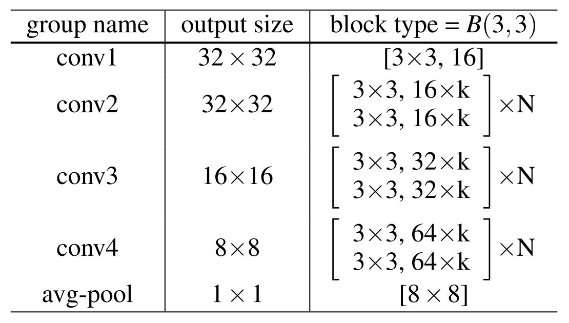
The wide resnet consists of three main architectural components:
- An initial convolution. This is done to pull out any high level features and help upsample our initial image from only three channels to a high-dimensional convolutional activation.
- A number of “groups”. Each group will consists of a set of \(N\) residual blocks. More on this in a moment.
- A pooling and linear layer. This will downsample our convolutions and convert them into class predictions.
The real meat of the wide resnet will lie in the groups: that’s where all of our residual blocks will live. The original paper always used three groups in their experiments, but we will write our code to be modular to the number of groups.

There are a few considerations that will become key to implementing the blocks in each of our groups:
- Each block after the first will downsample the size of the activations. This means that the 32x32 activation block will shrink to 16x16. We’ll do this by setting the stride of the first convolution in the blocks to 2.
- Each group will double the number of filters from the previous group.
- The first block of each group will need to have a convolution in its shortcut to get it to the right dimensions for the addition operation.
So how wide will these convolutions be? Our initial convolution will turn our three channels into 16. The first group will multiply the number of channels by the widening factor \(k\), and every subsequent group will double the width of the convolutions. Essentially, the \(i\)th group will have \((16 \cdot k)\cdot 2^i\) filters in its convolutions (where \(i\) starts from 0).
Implementing the Wide ResNet
Now that the architecture is all settled, it’s time to write some code. I’m going to implement this in PyTorch, with a little help from the fastai library. Fastai is a fantastic library for quickly building high quality models. It’s also really helpful for automating the more mundane aspects of writing deep learning code, like building data loaders and training loops, which is what I’ll use it for here.
The implementation will be done piece by piece: starting with the basic block, then fleshing out the whole network, and finally building our data pipeline and training loop. You can find the complete implementation here.
Note: Some of this code is not going to be as tidy as it could be. In this article, I’m optimizing for understanding, not necessarily style or cleanliness.
The BasicBlock Class
Since the majority of the model will consist of basic residual blocks, it makes
sense to define a reusable component that we can fill our model with.
Fortunately, PyTorch makes this really easy by allowing us to subclass the
nn.Module class.
The full implementation of the BasicBlock class can be seen below:
class BasicBlock(nn.Module):
    def __init__(self, inf, outf, stride, drop):
        super().__init__()
        self.bn1 = nn.BatchNorm2d(inf)
        self.conv1 = nn.Conv2d(inf, outf, kernel_size=3, padding=1,
                               stride=stride, bias=False)
        self.drop = nn.Dropout(drop, inplace=True)
        self.bn2 = nn.BatchNorm2d(outf)
        self.conv2 = nn.Conv2d(outf, outf, kernel_size=3, padding=1,
                               stride=1, bias=False)
        if inf == outf:
            self.shortcut = lambda x: x
        else:
            self.shortcut = nn.Sequential(
                    nn.BatchNorm2d(inf), nn.ReLU(inplace=True),
                    nn.Conv2d(inf, outf, 3, padding=1, stride=stride, bias=False))

    def forward(self, x):
        x2 = self.conv1(F.relu(self.bn1(x)))
        x2 = self.drop(x2)
        x2 = self.conv2(F.relu(self.bn2(x2)))
        r = self.shortcut(x)
        return x2.add_(r)
A few things to note:
- After the first group, the first block of each group will need to downsample
the height and width of the convolutional activation. This can be done by
passing in a 2 to the
strideparameter when instantiating the firstBasicBlockof the group. - With the exception mentioned above, each convolution should preserve the width
and height of the convolutional activation. We achieve this by always using a
kernel_sizeof 3 and apaddingof 1. Additionally, since we’re using batchnorm, our convolutions don’t need a bias parameter, hencebias=False. - We follow the order of batchnorm -> relu -> convolution. Although the original batchnorm paper used a different order, this has since been shown to be more effective during training.
- If this is the first block in a group, we’re going to double the width via our
convolutions. In that case, the dimensions won’t match for the shortcut
connection, so
shortcutwill need it’s own convolution (preceeded by batchnorm and relu) to increase it to have widthoutf. Also, since we only double on the first block in a group, and we may be downsampling then too, we’ll need to use thestrideparameter in this convolution as well.
The WideResNet Class
Now that we have our BasicBlock implementation, we can flesh out the rest of
the wide resnet architecture.
class WideResNet(nn.Module):
    def __init__(self, n_grps, N, k=1, drop=0.3, first_width=16):
        super().__init__()
        layers = [nn.Conv2d(3, first_width, kernel_size=3, padding=1, bias=False)]
        # Double feature depth at each group, after the first
        widths = [first_width]
        for grp in range(n_grps):
            widths.append(first_width*(2**grp)*k)
        for grp in range(n_grps):
            layers += self._make_group(N, widths[grp], widths[grp+1],
                                       (1 if grp == 0 else 2), drop)
        layers += [nn.BatchNorm2d(widths[-1]), nn.ReLU(inplace=True),
                   nn.AdaptiveAvgPool2d(1), Flatten(),
                   nn.Linear(widths[-1], 10)]
        self.features = nn.Sequential(*layers)

    def _make_group(self, N, inf, outf, stride, drop):
        group = list()
        for i in range(N):
            blk = BasicBlock(inf=(inf if i == 0 else outf), outf=outf,
                             stride=(stride if i == 0 else 1), drop=drop)
            group.append(blk)
        return group

    def forward(self, x):
        return self.features(x)
You can see the outline of the architecture in the code. Right after we call the
super constructor, we initialize the first convolutional layer (conv1 in the
architecture table).
After the initial convolution, we calculate the widths (i.e. number of filters) in
each block, creating a list that will become our inf and outf parameters
during block construction. Then we construct each group in a for loop. If this
is the first group, we use stride=1 since this is the only time we don’t want
to decrease the width and height of the convolutional activations. Making a
group involves calling our _make_group helper function, which will construct
N instances of BasicBlock with the appropriate inf, outf, and stride
parameters.
Finally, we average pool our activations, turning each \(64 \cdot k\) convolutional activations into a single value, which is input to our last linear layer used for classification.
Data Loading and Training
Our model is locked and loaded, now we just need some data to feed it and a training loop to optimize it. Since this is the least interesting part of building a model, I’m going to rely heavily on the fastai library. Note that for this code to run, the library will need to be importable, which is most simply done by cloning the repository and then symlinking the library directory into the same directory that the model is in.
To start, we’ll set up our data folder and download our dataset via
torchvision.datasets. We’ll also convert the dataset to numpy arrays of
floating point values, and move the inputs between 0 and 1.
os.makedirs(PATH, exist_ok=True)
trn_ds = CIFAR10(PATH, train=True, download=True)
tst_ds = CIFAR10(PATH, train=False, download=True)
trn = trn_ds.train_data.astype('float32')/255, np.array(trn_ds.train_labels)
tst = tst_ds.test_data.astype('float32')/255, np.array(tst_ds.test_labels)
Now trn and tst are tuples containing our training and test inputs/outputs,
respectively. Next we’ll set up our preprocessing transformations using fastai.
sz, bs = 32, 128
stats = (np.array([ 0.4914 ,  0.48216,  0.44653]),
         np.array([ 0.24703,  0.24349,  0.26159]))
aug_tfms = [RandomFlip(), Cutout(1, 16)]
tfms = tfms_from_stats(stats, sz, aug_tfms=aug_tfms, pad=4)
Our inputs will be size 32x32, with batch size 128 (you may need to decrease
this depending on your hardware; this is the value used in the original paper).
We set up our tfms object to be a list of transformation for our inputs: we
normalize based on the known means and standard deviations, take a random crop
after padding each size 4 pixels, and randomly flip the image 50% of the time.
Additionally, we also use cutout, which will
randomly zero out a square in our input image. Here we set cutout to use 1
square of length 16.
Finally, we’ll put everything together by creating a dataset object, instantiating our model, and creating a learner object.
data = ImageClassifierData.from_arrays('data', trn, tst, bs=bs, tfms=tfms)
wrn = WideResNet(n_grps=3, N=4, k=10)
learn = ConvLearner.from_model_data(wrn, data)
Here we’re using a wide resnet with 3 groups, each group has four blocks, and a widening factor of 10. We’ll also let dropout be 0.3, which is the default we picked when we defined the class. This results in a 28-layer network and produced the best results for our dataset.
To train, we will follow the same training procedure outline in the original paper.
lr = 0.01
wds = 5e-4
for i, epochs in enumerate([60, 60, 40, 40]):
    learn.fit(lr, epochs, wds=5e-4 best_save_name=f'wrl-10-28-p{i}')
    lr /= 5
We train for 200 epochs, decreasing the learning rate by a fifth at certain
intervals. Fastai will automatically save the best performing model of each
phase in our data directory since we set the best_save_name parameter.
In my own tests, this model achieved a final test time accuracy of 95.84%. The current state of the art for CIFAR-10 is about 98% (though they also trained for 9 times as long). Not bad for less than 100 lines of code!
Conclusion
In this post, I walked through implementing the wide residual network. Leveraging PyTorch’s modular API, we were able to construct the model with just a few dozen lines of code. We also were able to skip past the mundane image processing and training loop using the fastai library.
Our final results got us almost 96% accuracy on a rather challenging dataset. We are within 2% of the best that anybody has ever done. While deep learning moves at breakneck speeds, often times papers will present ideas that are fairly straightforward to reimplement yourself. This isn’t always the case, like in some experiments that require absolutely enormous computational power. But in cases like the wide resnet, it can be really fun and extremely rewarding to recreate a paper’s experiments from scratch.