Reinforcement Learning: Playing Doom with PyTorch
This tutorial is adapted from the one on ViZDoom’s website. Additionally, the code used here is adapted from this tutorial, with substantial modification.
Machine learning allows us to program by example. We can present the algorithm with some data, potentially provide it some feedback, and then glean the results of our system. For image classification, we give the model some images and it learns to identify what object(s) are in that image. Tasks like this where the model only needs to find the “right answer” (i.e. supervised learning) have seen a lot of success, and have huge potential to automate mundane manual tasks. But is that all machine learning can do?
In this post, I’ll introduce some of the ideas fundamental to reinforcement learning, and how it differs from typical supervised learning. We will then examine up close one algorithm for solving reinforcement learning problems, known as Deep Q-learning. Then, we’ll implement Deep Q-learning to teach a neural network how to play a simple game of Doom using the ViZDoom environment and PyTorch.

What is Reinforcement Learning?
Reinforcement learning is a branch of machine learning where we try to teach the model to actually do something. The most famous example of reinforcement learning is the success of DeepMind’s AlphaGo and its variants. Rather than just predicting an answer, AlhpaGo is a reinforcement learning agent that learns to masterfully play the game of Go. It can’t just classify; it needs to sequentially interact with its environment – making moves and receiving its opponent’s moves – in such a way that it will be most likely to achieve its long-term goal of winning the game.
Even though Go is just a board game, programming a competent player is exceedingly difficult. And interestingly, the same framework used to design AlphaGo can be applied to nearly any other domain. This framework is known as the Markov Decision Process (MDP), and it allows us to rigorously and mathematically characterize a system for reinforcement learning (as well as other situations).
The Markov Decision Process
MDPs have several different formulations and variants. However, there are two critical components that are tacitly understood: the agent and the environment. The agent is the person or thing that is actually trying to perform the task. They make the decisions and carry out the actions. The environment is essentially everything else: the world around the agent, the rules of that world, and even other players can be abstracted out to the environment.
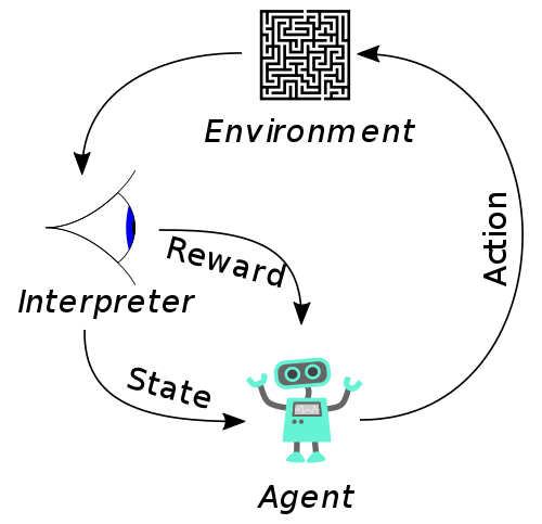
In addition to the agent and the environment, MDPs are made up of several pieces. First is the set of states, which is just the potential configurations of the agent/environment at a given point in time. For something like a board game, the state is just the current board and whether it’s the agent’s turn or not. Next are the actions: all the things that the agent can actually do. Note that the actions are dependent on the state, since not all actions are valid in every state. The last main piece is the reward function, which tells us how “good” our agent is doing at a task. This is what our reinforcement learning algorithm is going to focus on. Ultimately, we want to train the model to know how to act such that it will maximize the overall reward, also known as the return. The overall reward is calculated as just the sum of the rewards at each step in the process, but maximizing it is difficult, since we may have to make strategic decisions that are initially low reward to boost the final return.
Depending on the situation, the MDP may also include transition probabilities. These tell us how likely we are to transition to a new state \(s_2\) if we’re currently in a state \(s_1\) and we take some action \(a\). However, in complex problems we often don’t know what the transition probabilities will be. In a board game like Go, how can I effectively predict how my opponent will move? Additionally, in domains like Doom, the state space is so large that enumerating the transitions is impractical. So instead we let the reinforcement algorithm learn these transitions as well. Here is how reinforcement learning differs from planning systems: we don’t assume to know the world dynamics, and instead try to learn those dynamics along with good actions.
Aside: You may be wondering why we call this framework a Markov decision process. The Markov property states that we can reason about all future state given only the current state. That is, we only need to know where we are right now, not necessarily how we got here. This is usually the case, and is crucial for reinforcement learning algorithms to be tractable. Even in cases where the history is significant, there are ways we can encode that history into the current state to maintain the Markov property.
Deep Q-Learning
Up to this point, we’ve only described the reinforcement learning problem: given an MDP, we want to figure out good actions that will maximizes the sum of our rewards (i.e. the return). The process of deciding an action from a state is known as a policy, so in other words, we want to learn the best policy for a given task. There are several different algorithms that do this, but one of the most straightforward that we’ll look at here is known as Q-learning.
Before we can discuss how Q-learning actually works, we need some more terminology. Recall that the policy involves selecting an action from a state, and that the return is the sum over all our rewards at each state. Then the value of a state \(V_\pi(s)\) is the expected return if we start in state \(s\) and follow policy \(\pi\). Essentially, \(V_\pi\) tries to predict our final score using just the current state and the action-selection process.
We can take this a step further. Instead of taking just a state and trying to predict the final score, we can take the current state and an action and try to predict the return. This is known as the Q-value: \(Q_\pi(s, a)\). If our Q-values are accurate, then playing optimally just boils down to picking the action with the highest Q-value in our state. However, since we don’t know the transition probabilities, we have to estimate these Q-values, and try to improve them. This is where Q-learning comes in. Additionally, we can use deep neural networks to approximate the Q-functions, hence Deep Q-Learning.
You may have noticed that Q-functions are inherently recursive. That is, we can decompose the value of a Q-function by putting it in terms of the Q-function in the next state:
\[Q(s_t, a_t) = r_{t+1} + \gamma \cdot \max_a Q(s_{t+1}, a)\]where \(r_{t+1}\) is the reward we got for taking action \(a_t\), and \(\gamma\) is our discount factor that trades off immediate vs. long-term rewards. All this equation says is that Q-functions build off each other over time, and we can leverage that fact to efficiently estimate them.
To learn the Q-functions, we’ll utilize a deep neural network. The network will take a state as input, and output a vector of Q-values, one for each action. We will train it by presenting it with sets of transitions (a first state, action, reward, and second state). The Q-value for the first state should have a value in the index of the selected action that matches the right-hand side of the above equation. That difference (squared) will be our loss backpropagated through our network.
That’s really all there is to Deep Q-learning. We try to approximate a function that estimates our overall return after taking a particular action is a particular state. We turn this global problem into a much more localized variant by trying to optimize our Q-function estimations over individual transitions. Provided we have enough of these transitions and they are adequately diverse, the Q-function will converge to reasonably correct values that let us derive an optimal policy by repeatedly selecting the maximum action from the Q-values.
Putting it to Practice: ViZDoom
The ViZDoom environment is a fantastic tool for playing with reinforcement learning. It provides a nice programming interface for the classic video game Doom, and was designed with reinforcement learning in mind. It comes with several scenarios out of the box, such as the one we will use that involves shooting a monster across the room. However, these scenarios can actually be custom-built using existing free tools like Doom Builder.
For the sake of brevity, I’m only going to walk through the particularly important parts of the Q-learning implementation. You can see the full script to train and run the ViZDoom agent at this GitHub gist.
First, we’re going to define a class for our replay memory. The replay memory will serve as a bank of the recent transitions (e.g. first state, action taken, second state, and reward). Additionally, we need to keep track as to whether the action terminated the episode, since that will mean there is no second state to process.
class ReplayMemory:
    def __init__(self, capacity):
        channels = 1
        state_shape = (capacity, channels, *resolution)
        self.s1 = torch.zeros(state_shape, dtype=torch.float32).to(device)
        self.s2 = torch.zeros(state_shape, dtype=torch.float32).to(device)
        self.a = torch.zeros(capacity, dtype=torch.long).to(device)
        self.r = torch.zeros(capacity, dtype=torch.float32).to(device)
        self.isterminal = torch.zeros(capacity, dtype=torch.float32).to(device)

        self.capacity = capacity
        self.size = 0
        self.pos = 0

    def add_transition(self, s1, action, s2, isterminal, reward):
        idx = self.pos
        self.s1[idx,0,:,:] = s1
        self.a[idx] = action
        if not isterminal:
            self.s2[idx,0,:,:] = s2
        self.isterminal[idx] = isterminal
        self.r[idx] = reward

        self.pos = (self.pos + 1) % self.capacity
        self.size = min(self.size + 1, self.capacity)

    def get_sample(self, size):
        idx = sample(range(0, self.size), size)
        return (self.s1[idx], self.a[idx], self.s2[idx], self.isterminal[idx],
                self.r[idx])
The replay memory mostly just stores huge batches of the transitions, though we included some useful methods for adding transitions to the memory and gathering a random sampling from the non-zero entries. The replay memory will be critical to training our network, since it allows us to efficiently gather numerous and diverse inputs from the agent’s experience. In fact, the model will only learn from the replay memory directly. As the agent learns during training, it will leverage the Q-network to determine its actions, add its experience to the replay memory, and then update its parameters from a sample of transitions that come from the replay memory.
Next, we’ll build out our actual Q-function model. Recall that we are using a deep neural network to approximate our Q-function. Since ViZDoom will give us raw pixels as our inputs, we’ll leverage a convolutional neural net that can effectively learn the visual features.
class QNet(nn.Module):
    def __init__(self, available_actions_count):
        super(QNet, self).__init__()
        self.conv1 = nn.Conv2d(1, 8, kernel_size=6, stride=3) # 8x9x14
        self.conv2 = nn.Conv2d(8, 8, kernel_size=3, stride=2) # 8x4x6 = 192
        self.fc1 = nn.Linear(192, 128)
        self.fc2 = nn.Linear(128, available_actions_count)

        self.criterion = nn.MSELoss()
        self.optimizer = torch.optim.SGD(self.parameters(), FLAGS.learning_rate)
        self.memory = ReplayMemory(capacity=FLAGS.replay_memory)

    def forward(self, x):
        x = F.relu(self.conv1(x))
        x = F.relu(self.conv2(x))
        x = x.view(-1, 192)
        x = F.relu(self.fc1(x))
        return self.fc2(x)

    def get_best_action(self, state):
        q = self(state)
        _, index = torch.max(q, 1)
        return index

    def train_step(self, s1, target_q):
        output = self(s1)
        loss = self.criterion(output, target_q)
        self.optimizer.zero_grad()
        loss.backward()
        self.optimizer.step()
        return loss

    def learn_from_memory(self):
        if self.memory.size < FLAGS.batch_size: return
        s1, a, s2, isterminal, r = self.memory.get_sample(FLAGS.batch_size)
        q = self(s2).detach()
        q2, _ = torch.max(q, dim=1)
        target_q = self(s1).detach()
        idxs = (torch.arange(target_q.shape[0]), a)
        target_q[idxs] = r + FLAGS.discount * (1-isterminal) * q2
        self.train_step(s1, target_q)
Here we define the basic architecture and some useful methods for training. Note that the network isn’t particularly large: only 4 layers and not a great deal of parameters at each of those layers. The particular task isn’t very complex, and we’re restricting our inputs to small grayscale images of 30x45 pixels.
Pay particular attention to the second to last line in the learn_from_memory()
method. We want the Q-values for s1 to match the recursive equation above (but
only at the action that was actually taken during that transition). But updating
these indexes to the “true” value, we can take the squared difference as our
network loss.
Now that we have our replay memory and model, we can flesh out our training loop method. As I mentioned before, the basic formula is to first experience a transition, then record that transition and learn from the replay memory. Here’s the code below:
def perform_learning_step(epoch, game, model, actions):
    s1 = game_state(game)
    if random() <= find_eps(epoch):
        a = torch.tensor(randint(0, len(actions) - 1)).long()
    else:
        s1 = s1.reshape([1, 1, *resolution])
        a = model.get_best_action(s1.to(device))
    reward = game.make_action(actions[a], frame_repeat)

    if game.is_episode_finished():
        isterminal, s2 = 1., None
    else:
        isterminal = 0.
        s2 = game_state(game)

    model.memory.add_transition(s1, a, s2, isterminal, reward)
    model.learn_from_memory()
Note the action selection process. Initially, our agent has no idea what good
actions are. As such, we want it to explore very broadly, so that it can get a
diverse range of experience that it can build off of. The find_eps method will
determine some exploration rate depending on how far into training we are. As
the agent is more and more trained, it will take random actions (i.e. explore)
less and more often take the best action available. This is known as an
“epsilon-greedy” policy. When we’re done training, or evaluating our model, we
will always select the best action and no longer explore.
The rest of the code involves setting up the ViZDoom game, command line flags, and training epoch loops. All of it is pretty standard, and has thus been omitted. You can see and run the full script here. Since the network and inputs are pretty small, you should be able to run this on your personal computer, even if you don’t have a GPU.
I trained this model on my machine for 20 epochs at 2,000 iterations per epoch. Pretty quickly the agent learned a reasonable policy, and the whole thing converged in a little less than 20 minutes. You can see one of the test episodes in gif form below.
Additional Resources
Deep reinforcement learning is a burgeoning field with lots of exciting new advancements. This tutorial barely scratches the surface of Deep RL, but should provide you with everything to get started. If you’re interested in learning more, here are several resources that I found particularly interesting and/or useful.
- “Reinforcement Learning: An Introduction” by Sutton and Barto This is the textbook on reinforcement learning broadly. A classic in the field, and a free draft is available here.
- Reinforcement Learning Crash Course Lectures from David Silver’s course of reinforcement learning. Link
- “Deep Reinforcement Learning Doesn’t Work Yet” A critical yet honest appraisal of the current state of reinforcement learning and how it often falls short of our press releases. Link
- Deep Reinforcement Learning NIPS 2018 Workshop Collection of talks and papers literally on the cutting edge of Deep RL research (to be published with the conference in December). Link